SSD : Single Shot Multibox Detector(1)
원문 : https://arxiv.org/pdf/1512.02325.pdf
개요
이번 포스팅에서는 SSD : Single Shot Multibox Detector 논문을 공부합니다.
나는 사용했다 번역을 위해서 구글 번역기
12월 29일 수정중
22 Happy New Year
1월 01일 수정중
1월 15일 수정중
Abstract
SSD discretizes the output space of bounding boxes into a set of default boxes over different aspect ratios and scales per feature map location.
SSD는 피쳐 맵 위치당 서로 다른 종횡비 및 스케일에 대해 바운딩 박스의 출력 공간을 기본 상자 집합으로 구분합니다.
At prediction time, the network generates scores for the presence of each object category in each default box and produces adjustments to the box to better match the object shape
예측할 때, 신경망은 각 초기 박스에 있는 카테고리의 객체(존재)에 대해 점수를 내고 객체의 형태에 적합하도록 박스를 조절합니다.
SSD is simple relative to methods that require object proposals because it completely eliminates proposal generation and subsequent pixel or feature resampling stages and encapsulates all computation in a single network.
SSD는 제안 생성 및 후속 픽셀 또는 피쳐 재 샘플링 단계를 완전히 제거하고 단일 네트워크에서 모든 계산을 캡슐화하기 때문에 객체 제안이 필요한 방법에 비해 간단합니다.
1. Introduction
This paper presents the first deep network based object detector that does not resample pixels or features for bounding box hypotheses and and is as accurate as approaches that do
본 논문에서는 박스 가설을 위한 픽셀이나 특징을 리샘플링하지 않고 접근방법만큼 정확한 최초의 딥 네트워크 기반 객체 검출기를 제시한다.
The fundamental improvement inspeed comes from eliminating bounding box proposals and the subsequent pixel or feature resampling stage.
근본적인 개선 속도는 경계 상자 제안 및 후속 픽셀 또는 피쳐 리샘플링 단계를 제거하는 데서 비롯됩니다.
We introduce SSD, a single-shot detector for multiple categories that is faster thanthe previous state-of-the-art for single shot detectors (YOLO), and significantlymore accurate, in fact as accurate as slower techniques that perform explicit regionproposals and pooling (including Faster R-CNN).
싱글 샷 검출기(YOLO) 보다 빠르고 Faster R-CNN만큼 정확한 SSD를 소개합니다
The core of SSD is predicting category scores and box offsets for a fixed set of default bounding boxes using small convolutional filters applied to feature maps.
SSD의 핵심은 피쳐 맵에 적용되는 작은 컨볼류션 필터를 사용하여 고정된 기본 경계 상자 세트에 대한 카테고리 점수와 상자 오프셋을 예측하는 것입니다.
To achieve high detection accuracy we produce predictions of different scales from feature maps of different scales, and explicitly separate predictions by aspect ratio.
높은 검출 정확도를 달성하기 위해 우리는 다른 스케일의 특징 맵으로부터 다른 스케일의 예측을 생성하고 종횡비에 따라 명시 적으로 별개의 예측을 생성합니다.
요약
- SSD는 피쳐 맵을 서로 다른 스케일로 각각 예측해서 정확도가 높다.
2. The Single Shot Detector (SSD)
SSD 탐지 프레임워크를 설명하고 관련 훈련 방법과 데이터 세트 별 모델 세부 정보와 실험 결과를 제시

SSD only needs an input image and ground truth boxes for each object during training.
SSD는 훈련 중에 입력 영상과 진짜 상자만 대상으로 한다.
In a convolutional fashion,*
we evaluate a small set (e.g. 4) of default boxes of different aspect ratios at each location in several feature maps with different scales (e.g. 8 × 8 and 4 × 4 in (b) and (c)).
(b)와 (c) 사진 같이 서로 다른 스케일을 가진 피쳐 맵에서의 각 위치에서 서로 다른 종횡비의 작은 기본 상자 집합을 평가한다.
At training time, we first match these default boxes to the ground truth boxes. For example, we have matched two default boxes with the cat and one with the dog, which are treated as positives and the rest as negatives. The model loss is a weighted sum between localization loss (e.g. Smooth L1 [6]) and confidence loss (e.g. Softmax).
학습할 떄, 기본 상자들을 정답 레이블과 일치시킨다. 예시로 고양이와 기본 상자 두 개를, 개와 한 상자를 일치시켰는데 이것은 양성으로 취급되고 나머지는 음성으로 취급되나. 모델 손실은 위치 손실과 신뢰도 손실 값 사이의 가중치 합이다.
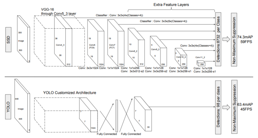
2.1 Model
The SSD approach is based on a feed-forward convolutional network that produces a fixed-size collection of bounding boxes and scores for the presence of object class instances in those boxes, followed by a non-maximum suppression step to produce the final detections.
SSD 접근 방식은 바운딩 박스의 고정크기 컬렉션과 해당 박스들의 객체 클래스 인스턴스의 존재에 대한 점수를 생성하는 feed-forward 컨볼류션 네트워크를 기반으로 한다.
최종 검출을 생성하기 위한 non-maximnum suppression 단계가 뒤따른다.
💡 offset ?
위치 좌표 주로 중심 x, y 좌표와 w, h, 너비와 높이
The early network layers are based on a standard architecture used forhigh quality image classification (truncated before any classification layers), which we will call the base network2.
초기 네트워크 계층은 고품질 이미지 분류에 사용되는 표준 아키텍처를 기반으로 하며 이것을 base network2라 부르겠다.
We then add auxiliary structure to the network to produce detections with the following key features:
그러고 네트워크에 보조적인 구조를 추가하여 아래와 같은 주요 특징들을 가진 탐지를 생성한다.
Key1 : Multi-scale feature maps for detection
We add convolutional feature layers to the endof the truncated base network.
잘린 기존 네트워크의 끝에 컨볼루션 특징 레이어를 추가한다.
These layers decrease in size progressively and allow predictions of detections at multiple scales.
이러한 레이어는 점차적으로 크기가 감소하고 여러 스케일에서 탐지를 예측할 수 있다.
The convolutional model for predicting detections is different for each feature layer
탐지를 예측하는 컨볼류선 모델은 각 특징 레이어마다 다르다
Key2 : Convolutional predictors for detection
in Each added feature layer (or optionally an existing feature layer from the base network) can produce a fixed set of detection predictions using a set of convolutional filters. These are indicated on top of the SSD network architecture in Fig. 2.
각각의 추가된 피쳐 레이어에서는, 컨볼류션 필터 세트를 사용해 고정된 탐지 예측 세트를 생성할 수 있다.
이는 SSD 네트워크 구조(그림2)에서 볼 수 있다.
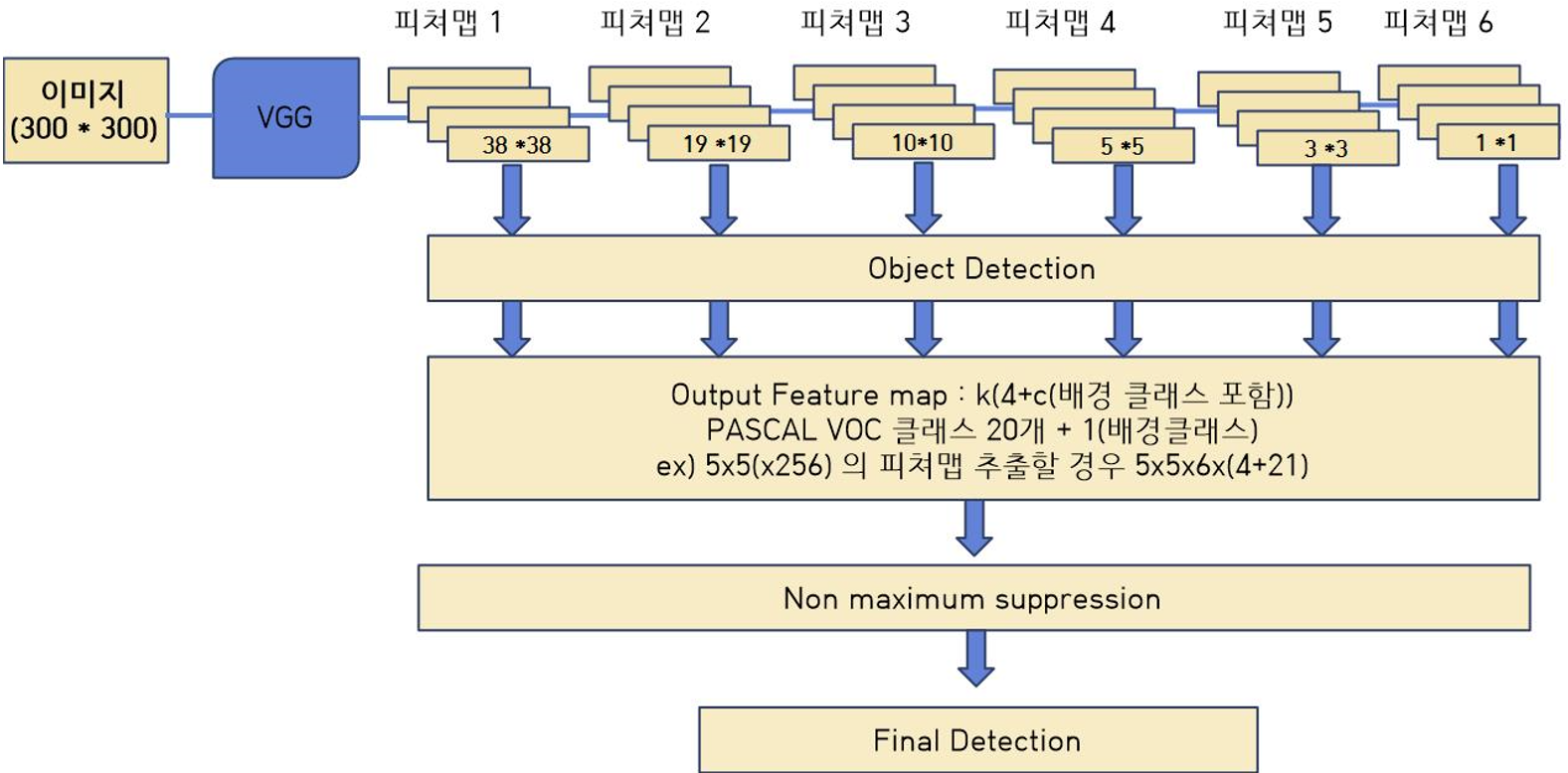
For a feature layer of size m × n with p channels, the basic element for predicting parameters of a potential detection is a 3 × 3 × p small kernel that produces either a score for a category, or a shape offset relative to the default box coordinates.
p 채널이 있는 m * n 크기의 피쳐 레이어의 경우,
잠재적 탐지의 매개변수를 예측하는 기본적인 요소는 3 * 3 * p 의 작은 커널이다.
이 커널은 카테고리에 대한 점수 또는 기본 상자 좌표에 대한 a shape offset relative을 생성한다.
At each of the m × n locations where the kernel is applied, it produces an output value.
커널이 적용되는 m * n의 각 위치에서 아웃풋 값을 생성한다.
The bounding box offset output values are measured relative to a default
경계 박스 오프셋 출력 값은 기본값에 대해 측정된다.
Our SSD model adds several feature layers to the end of a base network, which predict the offsets to default boxes of different scales and aspect ratios and their associated confidences.
우리 SSD 모델은 기존 신경망의 말단에 피쳐 레이어를 추가한 것으로, 다른 스케일의 디폴트 박스에 대한 오프셋, aspect 비율 그리고 관련된 confidence를 예측합니다
SSD with a 300 × 300 input size significantly outperforms its 448 × 448 YOLO counterpart in accuracy on VOC2007 test while also improving the speed
300 * 300 입력 크기를 가진 SSD는 VOC2007 테스트에서 정확도가 입력 크기가 448인 YOLO보다 현저히 뛰어나며 속도도 빠르다.
Default boxes and aspect ratios We associate a set of default bounding boxes with each feature map cell, for multiple feature maps at the top of the network.
디폴트 상자 및 종횡비 , 디폴트 경계 상자 집합을 각 피쳐 맵 셀과 연결하여 네트워크 상단의 여러 피쳐 맵에 대해 설명합니다.
The default boxes tile the feature map in a convolutional manner, so that the position of each box relative to its corresponding cell is fixed
디폴트 상자는 특징 맵을 컨볼류선 방식으로 타일 화하여 해당 셀과 관련된 각 상자의 위치가 고정되도록 합니다.
At each feature map cell, we predict the offsets relative to the default box shapes in the cell, as well as the per-class scores that indicate the presence of a class instance in each of those boxes.
각 피쳐 맵 셀에서, 셀의 기본상자와 관련된 오프셋과 해당 상자마다 클래스 인스턴스가 있음을 나타내는 클래스별 점수를 예측합니다.
Specifically, for each box out of k at a given location, we compute c class scores and the 4 offsets relative to the original default box shape.
구체적으로, 주어진 위치 k에서 각 상자에 대해, 우리는 원래 디폴트 박스 모양에 비해 c 클래스 점수와 4 오프셋을 계산한다.
This results in a total of (c + 4) k filters that are applied around eachlocation in the feature map, yielding (c + 4) kmn outputs for a m × n feature map.
이로 인해 특징 맵의 각 위치에 적용되는 총 (c + 4)k 필터가 생성되어 m* n 특징 맵에 대한 (c + 4) k*m*n 출력이 생성됩니다.
요약
2.2 Training
The key difference between training SSD and training a typical detector that uses region proposals, is that ground truth information needs to be assigned to specific outputs in the fixed set of detector outputs.
SSD와 다른 디텍터를 훈련하는데 있어 핵심 차이점은 고정된 검출기 출력 세트의 특정 출력에 데이터 원본을 할당해야 한다는 것입니다.
Matching strategy
During training we need to determine which default boxes correspond to a ground truth detection and train the network accordingly.
훈련중에 어떤 기본 상자가 원본에 해당하는지 결정하고 그에 따라 네트워크를 훈련시켜야 한다.
For each ground truth box we are selecting from default boxes that vary over location, aspect ratio, and scale.
각 본래 데이터의 박스에 대해 위치, 종횡비와 스케일에 따라 달라지는 기본 박스를 선택한다
We begin by matching each ground truth box to the default box with the best jaccard overlap (as in MultiBox [7]).
원본 데이터 박스를 디폴트 박스에 최상의 재 카드 오버랩(멀티박스 [7]에서와 같이)으로 매칭 시킨다.
Unlike MultiBox, we then match default boxes to any ground truth with jaccard overlap higher than a threshold (0.5).
멀티박스와 달리, 우리는 디폴트 박스를 임계값 0.5 보다 더 높은 재카드 오버랩을 일치시킨다.
This simplifies the learning problem, allowing the network to predict high scores for multiple overlapping default boxes rather than requiring it to pick only the one with maximum overlap.
네트워크가 최대 중복이 있는 상자만 선택하도록 요구하기보다는 여러 겹치는 기본 상자에 대해 높은 점수를 예측할 수 있게 학습 문제를 단순화한다
Choosing scales and aspect ratios for default boxes
we use both the lower and upper feature maps for detection.
탐지를 위해 하부, 상부 피쳐맵 모두를 사용한다.
Hard negative mining
After the matching step, most of the default boxes are negatives, especially when the number of possible default boxes is large.
매칭 단계 이후, 대부분의 디폴드 박스는 음수 값이다, 특히 디폴트 박스수가 클 때 더욱 마이너스다.
Instead of using all the negative examples, we sort them using the highest confidence loss for each default box and pick the top ones so that the ratio between the negatives and positives is at most 3:1.
모든 음수 값을 사용하는것 대신에, 각 디폴트 박스마다 가장 높은 confidence loss을 사용해 그들을 정렬하고 상위 상자를 선택하여 음과 양의 비율이 최대 3 : 1이 되도록 한다.
Data augmentation
To make the model more robust to various input object sizes and
shapes, each training image is randomly sampled by one of the following options
모델을 다양한 입력 객체 크기 및 모양에 보다 견고하게 만들기 위해 각 학습 이미지는 다음 옵션 중 하나에 의해 무작위로 샘플링됩니다.
1. 전체 원본 입력 이미지를 사용
2. 무작위로 패치를 샘플링합니다. 각 샘플링 패치의 크기는 [0]
3. 최소 자카드가 객체와 겹치도록 패치 샘플을 0.1, 0.3,0.5, 0.7 또는 0.9로 표시
'논문' 카테고리의 다른 글
| [논문 공부] Transformer : Attention IS All YOU NEED (0) | 2022.07.25 |
|---|---|
| [논문 공부] LSTM(Long Short-Term Memory)(feat. RNN) (0) | 2022.07.16 |
| [논문 공부] Sequence to Sequence Learning with Neural Networks (0) | 2022.07.11 |
| [모델공부]U-Net : Image segmentations (0) | 2022.01.10 |
| [모델구현]Unet 네트워크 구현하기(with Pytorch) (1) | 2022.01.09 |


